Study Guide
STOR 155 Guide: How Sampling, Regression, Confidence Intervals, and Hypothesis Tests Fit Together
Strong statistical conclusions come from a connected chain: how the data were generated, what the variables represent, which model fits the question, how uncertainty is measured, and how carefully the result is interpreted.
By DomyClass
Published:
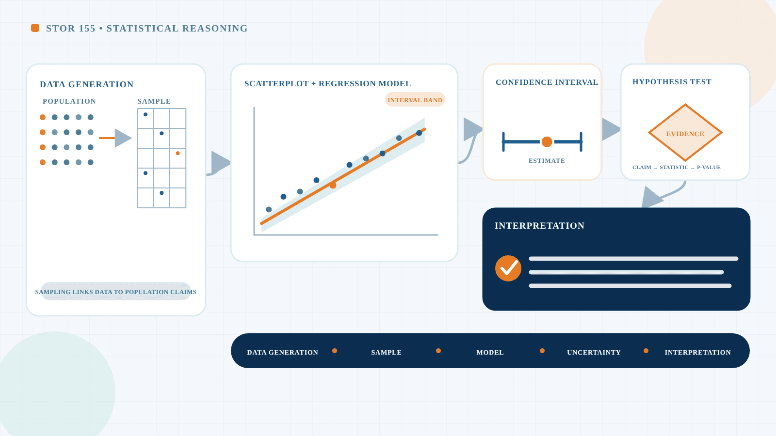
At a glance
Statistical methods work as a chain. A calculation near the end cannot repair a weak data source or a mismatched question near the beginning. Use these six checkpoints to keep the complete analysis visible.
Data-generation process
Identify how units were selected, what was measured, and whether conditions were observed or assigned.
Variable roles
Define the observational unit, distinguish categorical from quantitative variables, and name explanatory and response roles when relevant.
Sampling and design
Decide which population the sample can represent and whether the design supports association or a causal comparison.
Data model
Choose a probability or regression model that reflects the outcome, relationship, and assumptions in the question.
Estimate or test
Calculate a parameter estimate, an uncertainty interval, or a test statistic that answers the stated question.
Interpretation
Explain direction, magnitude, uncertainty, evidence, practical meaning, and limitations in ordinary language.
Start with the question, not the formula
A statistical analysis needs a target before it needs a procedure. State the research question in terms of a population, an outcome, and a comparison or relationship. The population is the full group or process of interest; the sample contains the units actually observed. A parameter is an unknown numerical feature of the population, while a statistic is calculated from the sample to estimate it.
Next define the observational unit represented by each row. In a study of public charging stations, one row might represent a station visit rather than a person or a day. If the question asks whether queue length helps predict waiting time, queue length is explanatory and waiting time is the response. These roles organize the model, but they do not establish cause. Writing the target first makes it easier to detect when the available data answer a narrower or different question.
How sampling affects inference
Population claims depend on how observations were selected. A representative sampling process gives the important kinds of population units an appropriate chance to appear. Random sampling helps prevent systematic selection patterns and provides a probability basis for sampling error. Sampling variability remains because two random samples will not be identical, so estimates change from sample to sample.
Selection bias is different from ordinary random variation. Suppose a city estimates charging-station wait times using only visits recorded during staffed daytime hours. Thousands of records may produce a very precise daytime estimate while missing overnight and weekend behavior. Enlarging the same biased collection process narrows random uncertainty around an incomplete target; it does not restore the missing visits. Before generalizing, explain who could enter the sample, who could not, and why that matters for the population named in the conclusion.
Observational studies and experiments
An observational study measures existing conditions without assigning them. It can reveal an association, but confounding may offer another explanation. Imagine comparing waiting times at charging stations that independently chose whether to display a live queue estimate. Stations adopting the display may also have newer equipment, different traffic, or more staff. A difference in waiting time cannot automatically be attributed to the display.
An experiment assigns a condition and compares responses. Random assignment helps distribute background characteristics across groups over repeated experiments, making a treatment comparison more credible. Random sampling and random assignment are not interchangeable: sampling addresses population representation, while assignment addresses causal comparison. An experiment conducted on a narrow volunteer group can support a treatment effect for that setting without automatically representing every station or visitor. The conclusion must preserve both boundaries.
Probability as the bridge
Probability links observed data to uncertainty. A random variable assigns a number to each possible outcome, and its expected value describes the model’s long-run center. Variability describes how widely outcomes are distributed around that center. Neither quantity predicts the exact next observation.
A normal model can represent continuous, roughly symmetric variation or the sampling behavior of an estimator under appropriate conditions. A binomial model represents a count of one defined outcome across a fixed number of comparable trials when its probability is stable and the needed independence condition is reasonable. Models simplify reality so that variation can be quantified; they do not reproduce every feature of a process. State what the model treats as random and check whether its assumptions make sense before using its probabilities for inference.
Correlation and regression
Begin with a scatterplot. Look for direction, form, strength, clusters, changing spread, and unusual points. Correlation summarizes the direction and strength of a linear association, but it can hide curvature and can change sharply because of an outlier. Association does not establish causation.
A regression line predicts the response from the explanatory variable. Its slope describes the modeled response change for a one-unit explanatory increase, and its intercept is the prediction when the explanatory value is zero. The intercept may have little practical meaning when zero is outside the observed range. A residual is the observed response minus its prediction; residual patterns can reveal curvature, uneven variability, or missing structure.
Prediction is safest in the range and setting represented by the data. Extrapolating beyond observed explanatory values assumes the pattern continues where it has not been checked. Report a prediction with its uncertainty and design limits rather than treating the fitted line as a universal rule.
From estimates to confidence intervals
A point estimate gives one sample-based value for an unknown parameter. Its standard error describes how much that estimator would vary across repeated samples under the model. A confidence interval adds and subtracts a margin of error based on the standard error and selected confidence level.
Suppose a random sample of station visits estimates the population mean waiting time at 11.4 minutes, with a 95% confidence interval from 10.6 to 12.2 minutes. A practical interpretation is that the method produces a range of plausible values for the population mean under the sampling and model assumptions. It is not correct to say that 95% of individual waits fall in the interval or that the completed interval has a 95% probability of containing the fixed mean.
Precision does not remove bias. Read the interval in context, ask whether its values would lead to different practical conclusions, and retain limitations from selection, measurement, and model choice.
From claims to hypothesis tests
A null hypothesis states a specific population or model condition; the alternative states the competing possibility. A test statistic compares the observed estimate with the null value in units of modeled uncertainty. The p-value is the probability, under the null model and test assumptions, of a statistic at least as incompatible with that model as the one observed.
This calculation does not assign a probability to the truth of the null hypothesis, quantify the effect, or establish practical importance. A threshold chosen as part of the plan can define a reject or fail-to-reject decision, but crossing that line is evidence rather than proof. Failing to reject may reflect a small effect, noisy data, limited information, or a null model reasonably compatible with the observations; it does not establish that the effect is absent.
A complete explanation reports the estimate, p-value when relevant, uncertainty, assumptions, and consequences. A statistically detectable difference may be too small to matter, while an inconclusive result may still allow effects important enough to study further.
Why confidence intervals and tests belong together
A hypothesis test asks how the data compare with a particular null value. A confidence interval displays a range of parameter values compatible with the data and method. For many standard two-sided procedures, a matching interval and test lead to corresponding decisions when they use the same assumptions and error level. That relationship is not a universal shortcut across every model, one-sided question, or adjusted analysis.
Use the test to describe evidence against the specified null and the interval to show magnitude and precision. Together they prevent a threshold decision from hiding the size of the effect or the range of values still supported by the data.
Means, proportions, and regression parameters
The target parameter determines what the result means, but it does not select a method by itself. Design, variable structure, dependence, sample behavior, and assumptions still need review.
| Target parameter | Example question | Typical estimate | Uncertainty output | Interpretation caution |
|---|---|---|---|---|
| Population mean | What is the mean wait for the target population of visits? | Sample mean | Standard error and confidence interval for the mean | The sampling process must support the population claim; the interval is not a range for most individual observations. |
| Population proportion | What share of target visits exceeds a defined wait threshold? | Sample proportion | Standard error and confidence interval for the proportion | Define the outcome and denominator precisely, and check model conditions rather than relying on sample size alone. |
| Regression slope | How does predicted waiting time change with queue length in the modeled range? | Estimated slope | Coefficient standard error and confidence interval | A slope is model-dependent association unless the study design supports a causal interpretation. |
Spreadsheet workflow
Spreadsheet software can make a statistical workflow transparent when raw observations, definitions, calculations, and checks remain visible. Use this sequence before writing the conclusion.
1. Preserve raw data.
2. Define variable roles.
3. Check missing and invalid values.
4. Calculate summaries.
5. Plot the data.
6. State the model.
7. Check assumptions.
8. Calculate the estimate or test.
9. Verify formulas and ranges.
10. Interpret in context.
Verification includes checking the sample count, units, cell ranges, copied formulas, category definitions, and a few calculations independently. A correctly evaluated formula is not enough when it refers to the wrong rows or answers the wrong question.
Common interpretation errors
Correlation means causation
Correlation describes linear association. Causation requires design support and consideration of confounding and alternative explanations.
Treating a p-value as odds that the null is correct
A p-value is calculated under the null model; it does not assign a probability to that hypothesis.
Nonsignificant means no effect
Failing to reject can leave a wide range of effects compatible with the data, especially when information is limited.
Significant means important
Statistical detectability does not measure practical value. Inspect the estimate, interval, and context.
A confidence interval contains most observations
An interval for a parameter addresses uncertainty in that parameter, not the spread of individual values.
A bigger sample fixes biased design
More observations can reduce random error while leaving systematic selection or measurement bias intact.
Regression is safe outside the observed range
Extrapolation assumes a relationship continues where no data verify it and should be clearly limited.
A unified STOR 155 reasoning framework
Use the framework as a loop rather than a one-way assembly line. A residual pattern may send you back to the model, a missing-data pattern may send you back to data generation, and an unclear conclusion may reveal that the original question needs a more precise target.
- Question
- Data generation
- Variables
- Visualize
- Model
- Assumptions
- Estimate or test
- Uncertainty
- Interpretation
- Limitations
At each stage, ask whether the next step answers the same question. The model should match the variables and design; the calculation should target the named parameter; the interpretation should preserve uncertainty; and the limitations should state what selection, measurement, or assumptions prevent you from claiming. This continuity is more important than memorizing isolated procedure names.
Related DomyClass resources
Continue with the STOR 155 and UNC-Chapel Hill hubs, or compare a focused explanation of the same statistical idea in another DomyClass course resource.
Turn this reasoning framework into an exam-preparation plan
Review STOR 155 topics, difficulty, the STOR 120 comparison, and a focused seven-day study plan.
Explore Turn this reasoning framework into an exam-preparation planSTOR 155 Introduction to Data Models and Inference
Return to the complete STOR 155 course-help hub and its topic overview.
Explore STOR 155 Introduction to Data Models and InferenceUniversity of North Carolina at Chapel Hill course resources
Browse the UNC-Chapel Hill institution hub and its available course support.
Explore University of North Carolina at Chapel Hill course resourcesMATH120 Introduction to Statistics
Foundational work with data, sampling, distributions, summaries, and uncertainty.
Explore MATH120 Introduction to StatisticsMAT-240 Applied Statistics
Applied hypothesis testing, correlation, regression, and interpretation.
Explore MAT-240 Applied StatisticsMATH302 Statistics
Probability, inference, assumptions, and statistical verification.
Explore MATH302 StatisticsDSRT 734 Inferential Statistics in Decision-Making
Graduate-level research design, inferential decisions, and interpretation.
Explore DSRT 734 Inferential Statistics in Decision-MakingSampling bias and representativeness
See why a large sample can still give a weak population claim when selection is biased.
Explore Sampling bias and representativenessHypothesis testing in plain English
Follow the path from a null model to a bounded evidence statement.
Explore Hypothesis testing in plain EnglishP-values, confidence intervals, and effect sizes
Keep statistical evidence, precision, and practical importance distinct.
Explore P-values, confidence intervals, and effect sizesAll DomyClass resources
Explore the complete directory of course hubs, study guides, and learning resources.
Explore All DomyClass resourcesSources
Course identity comes from current UNC-Chapel Hill sources. Statistical explanations draw on relevant sections of the NIST/SEMATECH e-Handbook of Statistical Methods and the American Statistical Association statement on p-values.
- Statistics and Operations Research (STOR)
University of North Carolina at Chapel Hill
- Undergraduate Courses
UNC Statistics and Operations Research
- Department of Statistics and Operations Research
University of North Carolina at Chapel Hill
- What Is EDA?
National Institute of Standards and Technology
- The Data Are Randomly Sampled from the Process
National Institute of Standards and Technology
- What Is Experimental Design?
National Institute of Standards and Technology
- Scatter Plot
National Institute of Standards and Technology
- How Can I Tell If a Model Fits My Data?
National Institute of Standards and Technology
- Normal Distribution
National Institute of Standards and Technology
- Binomial Distribution
National Institute of Standards and Technology
- Confidence Limits for the Mean
National Institute of Standards and Technology
- American Statistical Association Releases Statement on Statistical Significance and P-Values
American Statistical Association
Get Help With STOR 155 Introduction to Data Models and Inference at University of North Carolina at Chapel Hill
Get targeted STOR 155 help and improve your grades.
Get STOR 155 Help